使用课程推荐的Octave进行编程实现,可以将Octave理解为开源版本的MATLAB
Ex1: Linear Regression
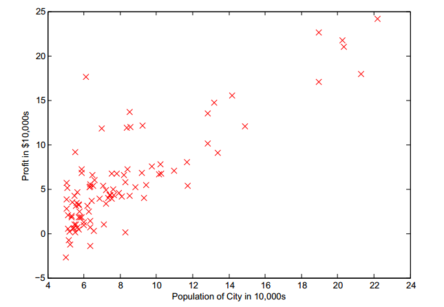
读入数据
1
2
3
4
5
6
data = load('ex1data1.txt'); % 导入的数据文件为用逗号隔开的两列,第一列为x,第二列为y
X = data(:, 1);
y = data(:, 2);
% 可以尝试绘图
% figure;plot(x,y);
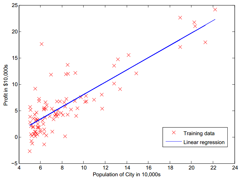
m = length(y);数据分布图如下:
梯度下降前的数据预处理与设置
1
2
3
4
5
6
X = [ones(m,1),data(:,1)]; % 添加x0列,都设为1
theta = zeros(2,1); % 初始化θ值
% 梯度下降的一些设置信息
iterations = 1500; % 迭代次数
alpha = 0.01; % 学习率α计算损失函数
线性回归的损失函数为:
1
2
3
4
5
6
7
% 定义一个函数computeCost来计算损失函数
function J = computeCost(X, y, theta)
m = length(y);
predictions = X*theta; % 计算预测值hθ
sqerrors = (predictions - y).^2; % 计算平方误,矩阵的点乘运算得到的是一个向量
J = 1/(2*m)* sum(sqerrors);
end执行梯度下降
1
2
3
4
5
6
7
8
9
10
11
12
13
% 定义一个函数gradientDescent来执行梯度下降,为了后面观察梯度下降过程中损失函数的变化,记录每一步迭代后的损失函数值
function [theta, J_history] = gradientDescent(X, y, theta, alpha, iterations)
m = length(y);
J_history = zeros(num_iters, 1);
% 以迭代次数为唯一迭代终止条件
for iter = 1:num_iters
% 计算梯度
predictions = X*theta;
updates = X'*(predictions - y);
theta = theta - alpha*(1/m)*updates;
J_history(iter) = computeCost(X, y, theta);
end
end绘制拟合直线
1
2
3
hold on; % 保留之前的绘图窗口,在这个绘图窗口继续画出拟合直线
plot(X(:,2), X*theta, '-');
legend('Training data', 'Linear regression');
Ex2: Logistic回归
目标:
构建一个logistics回归模型,依据学生两次考试的成绩来预测一个学生能否被大学录取
通过的输入数据文件为ex2data1.txt:
1 | # 为用逗号隔开的3列,分别为:exam1Score,exam2Score,lable |
读入数据,并画出数据分布散点图
1
2
3
4
5
6
7
8
9
10
11
12
13
14
15
16
17
18data = load('ex2data1.txt');
x = data(:,:2);
y = data(:,3);
% 画图
%% 区分出两类样本
pos = find(y==1);
neg = find(y==0);
figure;
%% 画出pos类样本
plot(x(pos,1), x(pos,2),'k+','MarkerSize', 3);
hold on;
%% 画出neg类样本
plot(x(neg,1), x(neg,2),'ko','MarkerSize', 3);
xlab('Exam 1 score');
ylab('Exam 2 score');
legend('Admitted', 'Not admitted');
hold off;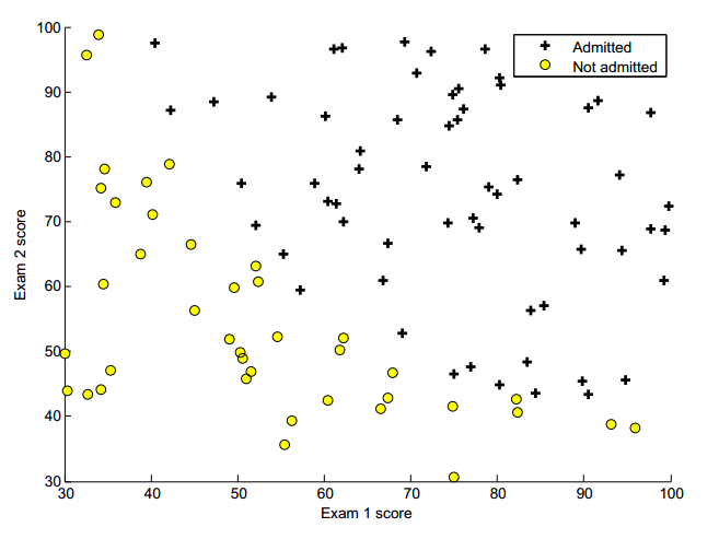
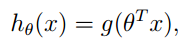
要得到的目标函数为 sigmoid 函数:

计算Cost和gradient
1
2
3
4
5
6
7
8
[m,n] = size(x);
X = [ones(m),data(:,:2)];
initialTheta = zeros(1,n+1);
% 计算初始的Cost和gradient
[initalCost,initialGradient] = costFunction(X,y,initialTheta);
% 打印出初始时的Cost和gradient
fprintf('Cost at initial theta(zeros): %f\n",initialCost);
fprintf('Gradient at initial theta(zeros): %f\n",initialGradient);在计算初始的Cost (initalCost) 和 gradient (initialGradient) 时,调用了自定义的函数costFunction
损失函数为:

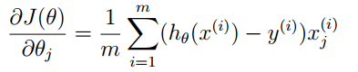
梯度的计算公式为:
下面给出costFunction函数的定义:
1
2
3
4
5
6
7
function [jVal,gradient] = costFunction(x,y,theta)
predict = sigmoid(x*theta);
leftCost = -y'*log(predict);
rightCost = -(1-y)'*log(1-predict);
jVal = (1/m)*(leftCost+rightCost);
gradient = (1/m)*((predict-y)'*x);
end在上面的costFunction函数中又调用了sigmoid函数,定义为:
1
2
3
function g = sigmoid(x)
g = 1./(1+exp(-x));
end优化目标函数
使其目标函数的Cost最小化,即

可以像练习一那样使用传统的梯度下降方法进行参数的优化,但Octave内部自带了
fminunc函数,可以用于非约束优化问题(unconstrained optimization problem)的求解fminunc函数的用法为:
1
2
3
4
5
6
7
%% 设置fminunc函数的内部选项
options = optmset('GradObj', 'on', 'MaxIter', 400);
% 'GradObj', 'on' 设置梯度目标参数为打开状态,即需要给这个算法提供一个梯度
% 'MaxIter', 400 设置最大迭代次数
%% 使用fminunc函数执行非约束优化
[optTheta, functionVal, exitFlag] = fminunc(@costFunction, initialTheta, options);一般情况下costFunction函数和它的函数名一样,只计算Cost值,不过由于这里要用到fminunc这个非约束优化函数,该函数需要提供Cost和gradient,所以在前面costFunction函数时,增加了一个计算梯度值的功能
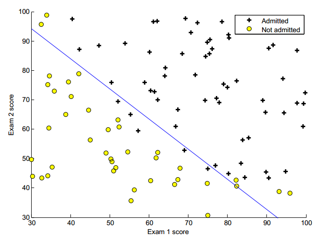
画出决策分界面 (Decision Boundary)
先像前面的第一步那样,画出原始数据分布散点图
1
2
3
4
5
6
7
8
9
10
11
% 画图
%% 区分出两类样本
pos = find(y==1);
neg = find(y==0);
figure;
%% 画出pos类样本
plot(x(pos,1), x(pos,2),'k+','MarkerSize', 3);
%% 画出neg类样本
plot(x(neg,1), x(neg,2),'ko','MarkerSize', 3);
xlab('Exam 1 score');
ylab('Exam 2 score');然后在散点图的基础上,把分界线画出来
分界线满足:
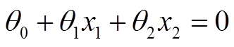
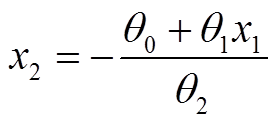
得到x1和x2直接的关系为:
1
2
3
4
5
6
7
hold on;
% 只需要选择两个点即可将直线画出
plot_x = [min(X(:,2))-2, max(X(:,2))+2];
plot_y = (-1./theta(3)).*(theta(2).*plot_x + theta(1));
plot(plot_x, plot_y)
legend('Admitted', 'Not admitted', 'Decision Boundary')
hold off;