1. 测序数据下载
参见: https://github.com/Ming-Lian/Memo/blob/master/ChIP-seq-pipeline.md#get-data
2. 比对与定量
2.1. Salmon流程
不需要比对,直接对转录水平进行定量
2.1.1. 创建索引
1 | $ salmon index -t Arabidopsis_thaliana.TAIR10.28.cdna.all.fa.gz -i athal_index_salmon |
2.1.2. 定量
salmon quant 有两种运行模式:
- Salmon’s quasi-mapping-based mode: using raw reads
输入以下命令查看该模式下的help文档
2
>
- Salmon’s alignment-based mode: makes use of already-aligned reads (in BAM/SAM format)
当使用参数
-a时,启用该模式,否则默认使用quasi-mapping-based mode输入以下命令查看该模式下的help文档
2
>
1 | #! /bin/bash |
salmon quant 参数:
- -i Salmon index
- -l Format string describing the library type.
-l Atells salmon that it should automatically determine the library type of the sequencing reads (e.g. stranded vs. unstranded etc.)- -1 File containing the #1 mates
- -2 File containing the #2 mates
- -p The number of threads to use
- -o Output quantification file.
2.2. subread流程
2.2.1. 创建索引
1 | $ gunzip Arabidopsis_thaliana.TAIR10.28.dna.genome.fa.gz |
2.2.2. 比对
1 | #! /bin/bash |
2.2.3. 定量
1 | featureCounts=~/anaconda2/bin |
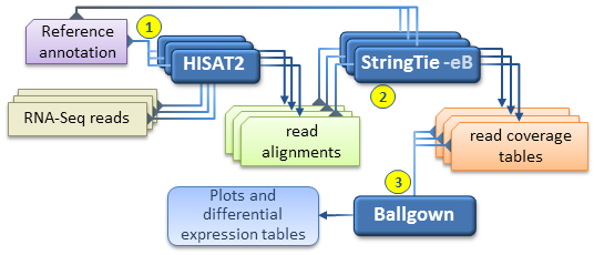
2.3. hisat2-stringtie流程
2.3.1. hisat2创建索引
1 | # build reference index |
2.3.2. hisat2比对
1 | $ hisat2 -p 10 --dta -x chrX_tran -1 reads1_1.fastq -2 reads1_2.fastq | samtools sort -@ 8 -O bam -o reads1.sort.bam 1>map.log 2>&1 |
Usage: hisat2 [options]* -x <ht2-idx> {-1 <m1> -2 <m2> | -U <r>} [-S <sam>]
- -p Number of threads to use
- –dta reports alignments tailored for transcript assemblers
- -x Hisat2 index
- -1 The 1st input fastq file of paired-end reads
- -2 The 2nd input fastq file of paired-end reads
- -S File for SAM output (default: stdout)
2.3.3. stringtie转录本拼接
1 | $ stringtie -p 16 -G Ref/hg19/grch37_tran/Homo_sapiens.GRCh37.75.gtf -o Asm/read1.gtf -l prefix Map/read1.bam 1>Asm/read1_strg_assm.log 2>&1 |
Transcript merge usage mode: stringtie --merge [Options] { gtf_list | strg1.gtf ...}
- -p number of threads (CPUs) to use
- -G reference annotation to include in the merging (GTF/GFF3)
- -o output path/file name for the assembled transcripts GTF
- -l name prefix for output transcripts (default: STRG)
2.3.4. stringtie定量
以ballgown格式输出
1
2$ stringtie -e -B -p 16 -G Asm/merge.gtf -o quant/read1/read1.gtf \
Map/read1.bam 1>quant/read1/read1_strg_quant.log 2>&1- -e only estimate the abundance of given reference transcripts (requires -G)
- -B enable output of Ballgown table files which will be created in the same directory as the output GTF (requires -G, -o recommended)
以read count进行定量,作为DESeq2或edgeR的输入
1
2
3$ stringtie -e -p 16 -G Asm/merge.gtf -o quant/read1/read1.gtf \
Map/read1.bam 1>quant/read1/read1_strg_quant.log 2>&1
$ python prepDE.py -i sample_lst.txt注意:
- stringtie的用法与上面相同,除了少了一个参数
-B prepDE.py脚本需要到stringtie官网下载:http://ccb.jhu.edu/software/stringtie/dl/prepDE.py ,注意该脚本是用python2编写的prepDE.py会以csv格式,分别输出基因和转录本的count matricesprepDE.py参数
- -i the parent directory of the sample sub-directories or a textfile listing the paths to GTF files [default: ballgown]
- -g where to output the gene count matrix [default: gene_count_matrix.csv]
- -t where to output the transcript count matrix [default: transcript_count_matrix.csv]
samplelist textfile 格式如下:
1
2
3
4
5
6
7
8
9
10ERR188021 <PATH_TO_ERR188021.gtf>
ERR188023 <PATH_TO_ERR188023.gtf>
ERR188024 <PATH_TO_ERR188024.gtf>
ERR188025 <PATH_TO_ERR188025.gtf>
ERR188027 <PATH_TO_ERR188027.gtf>
ERR188028 <PATH_TO_ERR188028.gtf>
ERR188030 <PATH_TO_ERR188030.gtf>
ERR188033 <PATH_TO_ERR188033.gtf>
ERR188034 <PATH_TO_ERR188034.gtf>
ERR188037 <PATH_TO_ERR188037.gtf>
- stringtie的用法与上面相同,除了少了一个参数
2.4. RSEM流程
RSEM属于Alignment-based transcript quantification的转录本定量工具的一种,也就是先比对后定量
RSEM最早被广泛应用于无参转录组的定量分析,因为无参转录组需要对reads进行拼接,然后将reads比对至拼接的转录本上,再通过定量获得其表达丰度
RSEM是在2010年发表的,最新更新是在2016年,下载地址则 http://deweylab.github.io/RSEM/,下载后编译下即可
1 | $ make |
RSEM整体上来说是属于定量软件,但其支持调用其他比对软件,如Bowtie,Bowtie2和STAR,来将reads比对至转录本上,所以必须至少预先安装上述3款比对软件中的一种,且要将它们的安装路径加入到环境变量PATH中
2.4.1. 创建索引
这步可以理解为是对转录本建索引,RSEM支持两种方式:
提供参考基因组fa序列和GTF注释文件
RSEM则会通过GTF注释文件从参考基因组序列中提取出各个转录本的序列,然后利用Bowtie2 or STAR等软件来建索引
2
3
4
5
> -gtf ~/annotation/hg38/gencode.v27.annotation.gtf \
> --bowtie2 \
> ~/reference/genome/hg38/GRCh38.p10.genome.fa ~/reference/index/RSEM/hg38/hg38
>
直接提供转录本序列,然后再建索引
无参转录组一般是这样的
参数与上面的情况相似,只是不需要设置
-gtf参数,若用户不指定-gtf参数,则RSEM会将后面提供的参考序列作为转录本如果还想有基于基因水平的定量结果,则需再加–transcript-to-gene-map参数,用于导入转录本和基因的对应关系的文件(一列基因ID,一列对应的转录本ID)
在~/reference/index/RSEM/hg38/目录下包含有从参考基因组提取出来的转录本的序列文件以及bowtie2的索引文件(以.bt2结尾)等
2.4.2. 转录本定量
用RSEM的rsem-calculate-expression命令来对reads进行bowtie2比对以及表达水平的定量
1 | $ ~/biosoft/rsem/RSEM-1.3.0/rsem-calculate-expression \ |
该命令有以下三种命令行形式:
1 | # 1. Single-end,比对与定量 |
参数说明:
–paired-end表明是双端测序数据–bowtie2指定bowtie2来用于reads比对–append-names用于在结果中附加上gene name和transcript name–output-genome-bam结果中输出基于基因水平的bam文件(默认只有转录水平的bam文件)–estimate-rspd文档中的例子还加了这个参数,用于estimate the read start position distribution,看是否有positional biases
RSEM通过调用bowtie2来完成mapping,其调用bowtie2时使用的默认参数为:
1 | $ bowtie2 \ |
也可以自己用bowtie2进行mapping将mapping得到的文件作为RSEM定量的输入,但是必须保证:
- 不支持有gap的比对
- 不支持paired reads discordant的比对
- 输出最佳的200个比对结果
否则RSEM会报错!
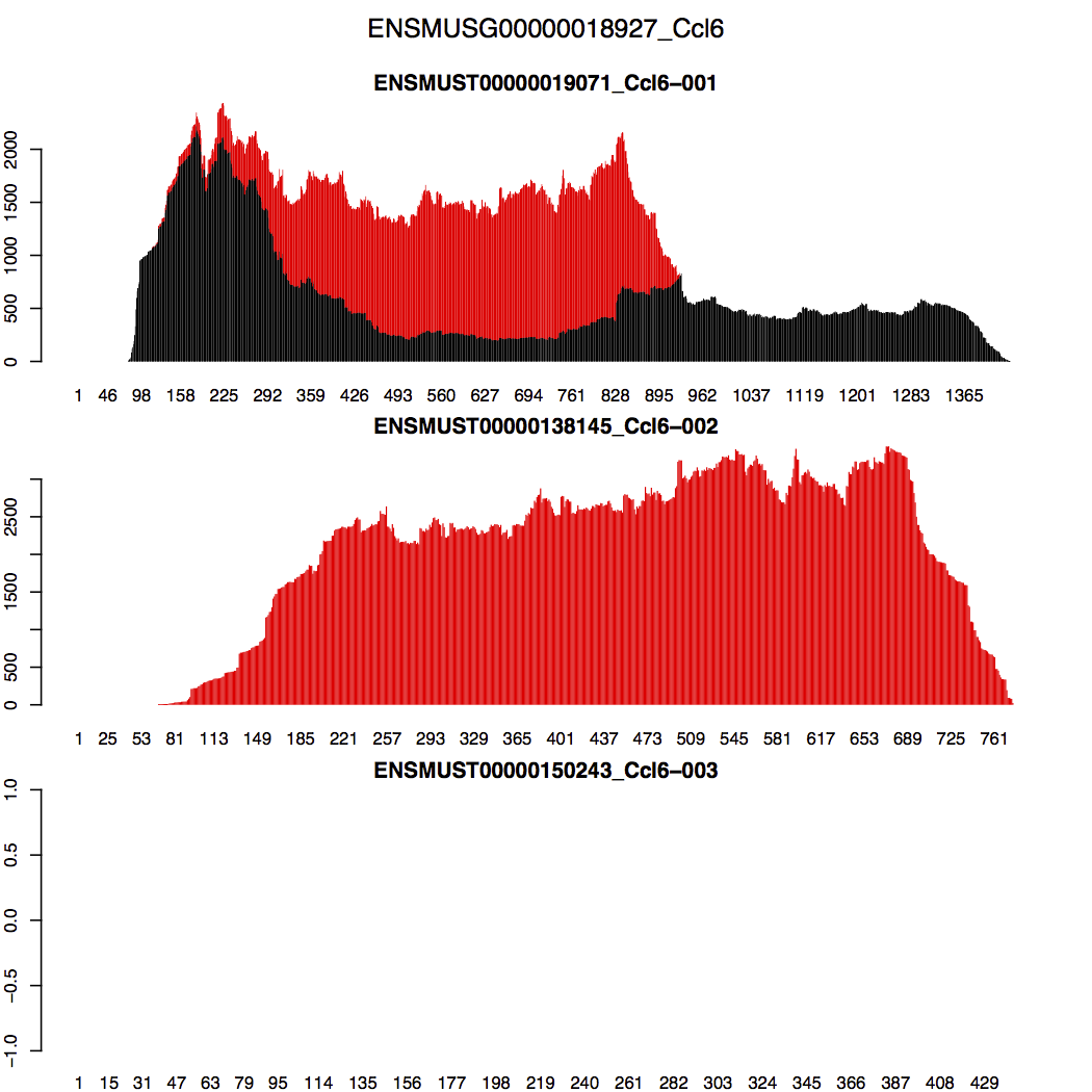
RSEM对multiple mapping结果的处理是这款工具的亮点:
对于RSEM如何处理multimapping reads,RSEM官方教程特意讲了一点
以Ccl6基因的3个转录本的比对结果为例,其第2个转录本全长与第1个转录本重叠,所以在这重叠区域会产生大量的multimapping reads,黑色表示uniquely aligned reads,红色表示multi-mapping reads
RSEM的处理方法是这样的:RSEM先尽量让第1个转录本在其重叠区域的reads(包括unique reads和multimapping reads)分布趋于平滑?因此再将在区域的剩下multimapping reads算在第2个转录本上;至于第3个转录本,其没有reads比对上,所以就空的;总体上如下图所示
3. 差异表达分析
3.1. 使用DESeq2进行差异分析
DESeq2要求输入的表达矩阵是read counts
构建 DESeqDataSet 对象
1 | # 构建表达矩阵 |
表达矩阵的格式为:
|
SRR1039508 | SRR1039509 | SRR1039512 | SRR1039513 | SRR1039516 | SRR1039517 | SRR1039520 | SRR1039521 | |
|---|---|---|---|---|---|---|---|---|---|
| ENSG00000000003 | 679 | 448 | 873 | 408 | 1138 | 1047 | 770 | 572 | |
| ENSG00000000005 | 0 | 0 | 0 | 0 | 0 | 0 | 0 | 0 | |
| ENSG00000000419 | 467 | 515 | 621 | 365 | 587 | 799 | 417 | 508 | |
| ENSG00000000457 | 260 | 211 | 263 | 164 | 245 | 331 | 233 | 229 | |
| ENSG00000000460 | 60 | 55 | 40 | 35 | 78 | 63 | 76 | 60 | |
| ENSG00000000938 | 0 | 0 | 2 | 0 | 1 | 0 | 0 | 0 | |
| ENSG00000000971 | 3251 | 3679 | 6177 | 4252 | 6721 | 11027 | 5176 | 7995 | |
| ENSG00000001036 | 1433 | 1062 | 1733 | 881 | 1424 | 1439 | 1359 | 1109 | |
| ENSG00000001084 | 519 | 380 | 595 | 493 | 820 | 714 | 696 | 704 | |
| ENSG00000001167 | 394 | 236 | 464 | 175 | 658 | 584 | 360 | 269 | |
| ENSG00000001460 | 172 | 168 | 264 | 118 | 241 | 210 | 155 | 177 | |
| ENSG00000001461 | 2112 | 1867 | 5137 | 2657 | 2735 | 2751 | 2467 | 2905 | |
| ENSG00000001497 | 524 | 488 | 638 | 357 | 676 | 806 | 493 | 475 | |
| ENSG00000001561 | 71 | 51 | 211 | 156 | 23 | 38 | 134 | 172 |
分组矩阵的格式为:
|
dex | SampleName | cell |
|---|---|---|---|
| SRR1039508 | untrt | GSM1275862 | N61311 |
| SRR1039509 | trt | GSM1275863 | N61311 |
| SRR1039512 | untrt | GSM1275866 | N052611 |
| SRR1039513 | trt | GSM1275867 | N052611 |
| SRR1039516 | untrt | GSM1275870 | N080611 |
| SRR1039517 | trt | GSM1275871 | N080611 |
| SRR1039520 | untrt | GSM1275874 | N061011 |
| SRR1039521 | trt | GSM1275875 | N061011 |
差异表达分析
1 | ## 数据过滤 |
3.2. 使用Ballgown进行差异分析
紧接着stringtie的定量结果进行分析
stringtie的定量结果提供多种表达值的表示方法,有read counts, RPKM/FPKM, TPM 。其中read counts是原始reads计算,RPKM/FPKM 和 TPM 都是基因表达值的归一化后的,因为本身的某些缺点,主流科学家强烈要求它就被TPM取代了。
下面对 RPKM/FPKM 和 TPM 的说明摘抄自健明大大的简书:https://www.jianshu.com/p/e9d5d7206124 ,说得通俗易懂
TPM是什么?
我不喜欢看公式,直接说事情,我有一个基因A,它在这个样本的转录组数据中被测序而且mapping到基因组了 5000个的reads,而这个基因A长度是10K,我们总测序文库是50M,所以这个基因A的RPKM值是 5000除以10,再除以50,为10. 就是把基因的reads数量根据基因长度和样本测序文库来normalization 。
那么它的TPM值是多少呢? 这个时候这些信息已经不够了,需要知道该样本其它基因的RPKM值是多少,加上该样本有3个基因,另外两个基因的RPKM值是5和35,那么我们的基因A的RPKM值为10需要换算成TPM值就是 1,000,000 *10/(5+10+35)=200,000, 看起来是不是有点大呀!其实主要是因为我们假设的基因太少了,一般个体里面都有两万多个基因的,总和会大大的增加,这样TPM值跟RPKM值差别不会这么恐怖的。
- 载入R包
1 | require(ballgown) |
- 载入stringtie输出的表达数据,并设置表型信息(即分组信息)
1 | bg_Z1Z4<-ballgown(dataDir="SingleCell_process/Cleandata/Expression",samplePattern=“Z[14]T",meas="FPKM") |
- 过滤低丰度的基因
1 | bg_Z1Z4_filt<-subset(bg_Z1Z4,"rowVars(texpr(bg_Z1Z4))>1",genomesubset=T) |
- 差异表达基因分析
1 | result_genes<-stattest(bg_Z1Z4_filt,feature="gene",covariate="group",getFC=T) |
分组设置对差异表达分析的影响:
- FC = group_1/group_0,所以分组标签互换后FC会变为原来的倒数
- 差异转录本分析
1 | result_trans<-stattest(bg_Z1Z4_filt,feature="transcript",covariate="group",getFC=T) |
4. 几点思考
- 为什么要进行转录本拼接?不是都有参考转录组了吗?
- 无参考基因组:对于无参考转录组的物种来说,往往需要通过RNA-Seq的数据自己拼出参考转录组,然后再进行下游的数据分析。所以,对于无参分析来说,往往需要自己拼装转录本,生成自己的参考转录组信息
- 注释完备的基因组:例如human,不同的细胞条件可能不同,一些永生化的细胞系往往都具有“癌症”的特征,这些细胞的转录组,基因组或多或少都有结构的变异,以及转录本的差异。
参考资料:
(1) 【PANDA姐的转录组入门】拟南芥实战项目-定量、差异表达、功能分析
(2) 一步法差异分析
(3) Pertea M, Kim D, Pertea G M, et al. Transcript-level expression analysis of RNA-seq experiments with HISAT, StringTie and Ballgown.[J]. Nature Protocols, 2016, 11(9):1650.
(4) Alignment-based的转录本定量-RSEM
(5) RSEM官方教程
(6) 知乎《高通量测序技术》专栏:生物信息学100个基础问题 —— 第25题 GTF/GFF的注释是怎么来的,应该从哪里下载?