
Schematic diagram of the MeRIP-seq protocol

由于m6A-seq数据分析的原理与过程和ChIP-seq十分相似,所以这里略过前面的质控,简单说明比对和peak calling步骤,具体内容可以参考ChIP-seq分析流程
m6A背景知识
目前已知有100多种RNA修饰,涉及到mRNAs、tRNAs、rRNAs、small nuclear RNA (snRNAs) 以及 small nucleolar RNAs (snoRNAs)等。其中甲基化修饰是一种非常广泛的修饰,N6-methyl adenosine (m6A)是真核生物mRNA上最为广泛的甲基化修饰之一,并存在于多种多样的物种中。
腺嘌呤可以被编码器METTL3、METTL14和WTAP及其他组分组成的甲基转移酶复合体甲基化,甲基化的腺嘌呤可以被读码器(目前发现m6A读码器主要有四个,定位于细胞核内的YTHDC1以及定位在细胞质中的YTHDF1、YTHDF2、YTHDF3、YTHDC2)识别,同时m6A可以被擦除器FTO和ALKBH5这两个去甲基化酶催化去甲基化。
在哺乳动物mRNA中,m6A修饰存在于7000多个基因中,保守基序为RRACH (R = G, A; H = A, C, U)。m6A修饰富集在mRNA终止密码子附近。
比对参考基因组
在 ChIP-seq 中一般用 BWA 或者 Bowtie 进行完全比对就可以了,但是在 MeRIP-seq 中,由于分析的 RNA ,那么就存在可变剪切,对于存在可变剪切的 mapping 用 Tophat 或者 Tophat 的升级工具 HISAT2 更合适
Tophat
1 | # build reference index |
Tophat参数
- -p Number of threads to use
- -G Supply TopHat with a set of gene model annotations and/or known transcripts, as a GTF 2.2 or GFF3 formatted file.
- –transcriptome-index TopHat should be first run with the -G/–GTF option together with the –transcriptome-index option pointing to a directory and a name prefix which will indicate where the transcriptome data files will be stored. Then subsequent TopHat runs using the same –transcriptome-index option value will directly use the transcriptome data created in the first run (no -G option needed after the first run).
- -o Sets the name of the directory in which TopHat will write all of its output
samtools view 参数
- -q only include reads with mapping quality >= INT [0]
HISAT2
1 | # build reference index |
Usage: hisat2 [options]* -x <ht2-idx> {-1 <m1> -2 <m2> | -U <r>} [-S <sam>]
- -p Number of threads to use
- –dta reports alignments tailored for transcript assemblers
- -x Hisat2 index
- -1 The 1st input fastq file of paired-end reads
- -2 The 2nd input fastq file of paired-end reads
- -S File for SAM output (default: stdout)
Peak calling
MACS2
参考ChIP-seq分析流程中的peak calling过程
PeakRanger
1 | peakranger ccat --format bam SRR1042594.sorted.bam SRR1042593.sorted.bam \ |
Peaks注释
CEAS
哈佛刘小乐实验室出品的软件,可以跟MACS软件call到的peaks文件无缝连接,实现peaks的注释以及可视化分析
CEAS需要三种输入文件:
- Gene annotation table file (sqlite3)
可以到CEAS官网上下载:http://liulab.dfci.harvard.edu/CEAS/src/hg18.refGene.gz ,也可以自己构建:到UCSC上下载,然后用
build_genomeBG脚本转换成split3格式- BED file with ChIP regions (TXT)
需要包含chromosomes, start, and end locations,这样文件可以由 peak-caller (如MACS2)得到
- WIG file with ChiP enrichment signal (TXT)
如何得到wig文件可以参考samtools操作指南:以WIG文件输出测序深度
CEAS的使用方法很简单:1
2
3ceas --name=H3K36me3_ceas --pf-res=20 --gn-group-names='Top 10%,Bottom 10%' \
-g hg19.refGene -b ../paper_results/GSM1278641_Xu_MUT_rep1_BAF155_MUT.peaks.bed \
-w ../rawData/SRR1042593.wig
- –name Experiment name. This will be used to name the output files.
- –pf-res Wig profiling resolution, DEFAULT: 50bp
- –gn-group-names The names of the gene groups in –gn-groups. The gene group names are separated by commas. (eg, –gn-group-names=’top 10%,bottom 10%’).
- -g Gene annotation table
- -b BED file of ChIP regions
- -w WIG file for either wig profiling or genome background annotation.
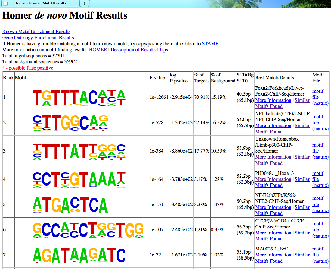
Motif识别
HOMER
安装旧版本的HOMER比较复杂,因为旧版依赖于调用其他几个工具:
- blat
- Ghostscript
- weblogo
Does NOT work with version 3.0!!!!
新版HOMER安装很简单,主要是通过configureHomer.pl脚本来安装和管理HOMER1
2
3
4
5
6
7
8
9cd ~/biosoft
mkdir homer && cd homer
wget http://homer.salk.edu/homer/configureHomer.pl
# Installing the basic HOMER software
perl configureHomer.pl -install
# Download the hg19 version of the human genome
perl configureHomer.pl -install hg19
安装好后可以进行 Motif Identification1
2
3
4
5
6
7
8
9
10
11
12
13
14# 提取对应的列给HOMER作为输入文件
# change
# chr1 1454086 1454256 MACS_peak_1 59.88
#to
# MACS_peak_1 chr1 1454086 1454256 +
$ awk '{print $4"\t"$1"\t"$2"\t"$3"\t+"}' macs_peaks.bed >homer_peaks.bed
# MeRIP-seq 中 motif 的长度为6个 nt
$ findMotifsGenome.pl homer_peaks.bed hg19 motifDir -size 200 -len 8,10,12
# 自己指定background sequences,用bedtools shuffle构造随机的suffling peaks
$ bedtools shuffle -i peaks.bed -g <GENOME> >peaks_shuffle.bed
# 用参数"-bg"指定background sequences
$ findMotifsGenome.pl homer_peaks.bed hg19 motifDir -bg peaks_shuffle.bed -size 200 -len 8,10,12
Usage: findMotifsGenome.pl <pos file> <genome> <output directory> [additional options]
注意:
<genome>参数只需要写出genome的序号,不需要写出具体路径bedtools shuffle中的genome文件的格式要求:
2
3
4
5
6
> chr1 249250621
> chr2 243199373
> ...
> chr18_gl000207_random 4262
>
可以使用 UCSC Genome Browser’s MySQL database 来获取 chromosome sizes 信息并构建genome文件
2
>
最后得到的文件夹里面有一个详细的网页版报告
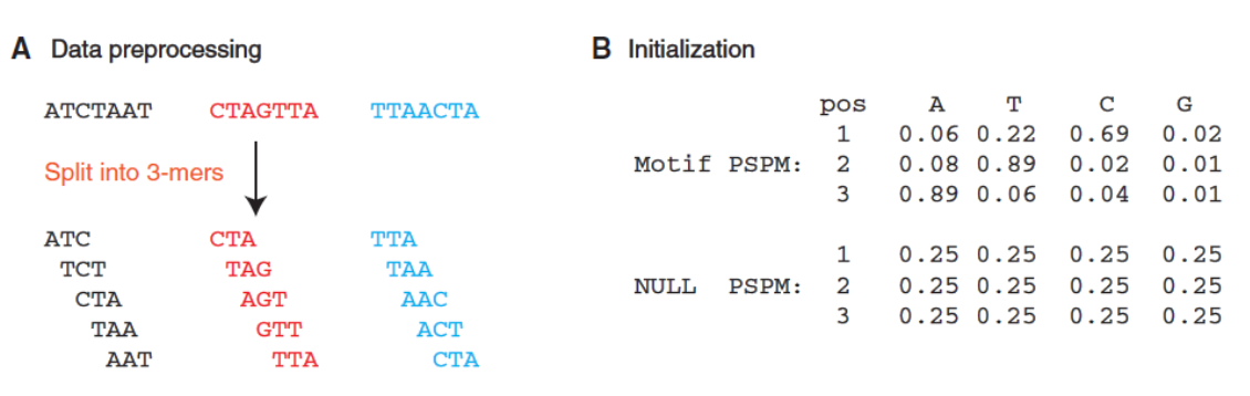
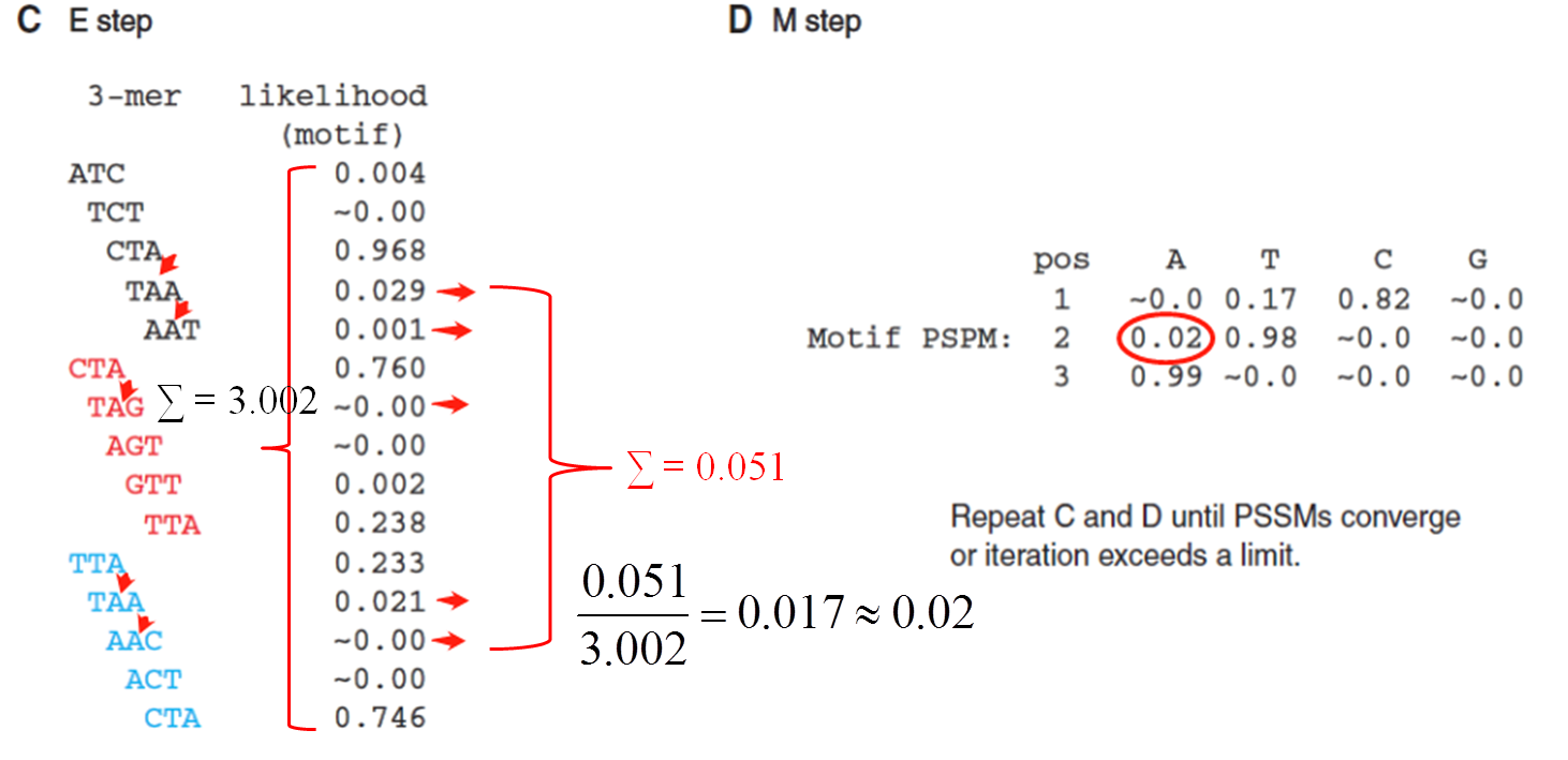
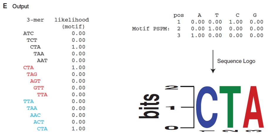
MEME
算法原理
操作
下载安装MEME
1 | cd ~/biosoft |
1 | # 先提取peaks区域所对应的序列 |
Usage: meme <dataset> [optional arguments]
- < dataset > File containing sequences in FASTA format
- -dna Sequences use DNA alphabet
- -mod Distribution of motifs,3 options: oops | zoops | anr
- -pal Force palindromes (requires -dna)
Differential binding analysis
Merge peaks
当ChIP-seq数据中有多分组,多样本以及多个重复时,需要进行样本间peaks的merge
1 | bedtools intersect -a Mcf7H3k27acUcdAlnRep1_peaks.filtered.bed -b Mcf7H3k27acUcdAlnRep2_peaks.filtered.bed -wa | cut -f1-3 | sort | uniq > Mcf7Rep1_peaks.bed |
Preparing ChIP-seq count table
用bedtools
1 | # Make a bed file adding peak id as the fourth colum |
- NR 表示awk开始执行程序后所读取的数据行数
- OFS Out of Field Separator,输出字段分隔符
用featureCounts (subread工具包中的组件)
1 | # Make a saf(simplified annotation format) file for featureCount in the subread package, |
Usage: featureCounts [options] -a <annotation_file> -o <output_file> input_file1 [input_file2] ...
- -a Name of an annotation file
- -F Specify format of the provided annotation file. Acceptable formats include ‘GTF’ (or compatible GFF format) and ‘SAF’. ‘GTF’ by default
- -o Name of the output file including read counts
- -T Number of the threads
Differential binding by DESeq2
- 对 contrast 构建一个 counts 矩阵,第一组的每个样本占据一列,紧接着的是第二组的样本,也是每个样本一列。
1 | # 做好表达矩阵 |
- 接着计算每个样本的 library size 用于后续的标准化。library size 等于落在该样本所有peaks上的reads的总数,即 counts 矩阵中每列的加和。如果bFullLibrarySize设为TRUE,则会使用library的总reads数(根据原BAM/BED文件统计获得)。然后使用
estimateDispersions估计统计分布,需要将参数fitType设为’local’
1 | dds<-estimateSizeFactors(dds) |
- 对负二项分布进行显著性检验(Negative Binomial GLM fitting and Wald statistics)
1 | dds <- nbinomWaldTest(dds) |
若存在多个分组需要进行两两比较,则需要提取指定的两个分组之间的比较结果1
2
3
4## 提取你想要的差异分析结果,我们这里是treated组对untreated组进行比较
res <- results(dds2, contrast=c("group_list","treated","untreated"))
resOrdered <- res[order(res$padj),]
resOrdered=as.data.frame(resOrdered)
注意两个概念:
Full library size: bam文件中reads的总数
Effective library size: 落在peaks区域的reads的总数
DESeq2中默认使用 Full library size bam (bFullLibrarySize =TRUE),在ChIP-seq中使用 Effective library size 更合适,所有应该设置为bFullLibrarySize =FALSE
4. Differential binding peaks annotation
在Differential binding analysis: 2. Preparing ChIP-seq count table得到的bed_for_multicov.bed中找DiffBind peaks的bed格式信息
1 | # 用R进行取交集操作 |
接着,用基因组注释文件GFF/GTF注释peaks
1 | $ bedtools intersect -wa -wb -a m6A_seq/CallPeak/peaks_diffBind.bed -b Ref/mm10/mm10_trans/Mus_musculus.GRCm38.91.gtf >m6A_seq/CallPeak/peaks_diffbind.anno.bed |
peaks注释基因的富集分析
clusterProfiler: GO enrichment analysis
多数人进行GO富集分析时喜欢使用DAVID,但是由于DAVID的最新版本是在2016年更新的,数据并不是最新的,所以不推荐使用DAVID。
推荐使用bioconductor包clusterProfiler
准备geneList
从DiffBind peaks annotation中获得的peaks_diffbind.anno.bed文件中提取geneID
1 | $ cut -f 13 m6A_seq/CallPeak/peaks_diffbind.anno.bed | \ |
1 | # 载入geneList,最终提供给enrichGO的gene list应该是一个geneID的向量 |
GO over-representation test
1 | # 需要使用到相应物种的基因组注释数据包(org.Xx.eg.db),请提前安装好,下面以老鼠为例 |
参数说明:
- gene: a vector of entrez gene id
- OrgDb: OrgDb
- keytype: keytype of input gene
- ont: One of “MF”, “BP”, and “CC” subontologies
- pvalueCutoff: Cutoff value of pvalue
- pAdjustMethod: one of “holm”, “hochberg”, “hommel”, “bonferroni”, “BH”, “BY”, “fdr”, “none”
- qvalueCutoff: qvalue cutoff
- readable: whether mapping gene ID to gene Name
1 | head(ego) |
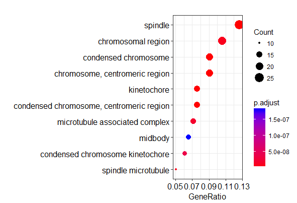
富集分析结果可视化
1 | # 绘制气泡图 |
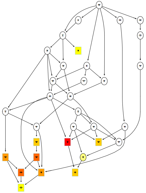
1 | # 绘制GOterm拓扑关系网,依赖topGO和Rgraphviz |
参考资料:
(1) Zhang C, Chen Y, Sun B, et al. m(6)A modulates haematopoietic stem and progenitor cell specification[J]. Nature, 2017, 549(7671):273.
(2) BIG科研 | 细胞质内的m6A结合蛋白YTHDF3促进mRNA的翻译
(3) Pertea M, Kim D, Pertea G, et al. Transcript-level expression analysis of RNA-seq experiments with HISAT, StringTie, and Ballgown[J]. Nature Protocols, 2016, 11(9):1650.
(5) ChIPseq pipeline on jmzeng1314’s github
(6) ChIPseq pipeline on crazyhottommy’s github
(7) library size and normalization for ChIP-seq
(8) Bioconductor tutorial: Analyzing RNA-seq data with DESeq2
(9) Bioconductor tutorial: clusterProfiler
(10) 国科大-韩春生《生物信息学应用 - 模序搜索》ppt